The Turing package for Julia provides a sweet way of doing Bayesian inference. Here I demonstrate how to do inference in a Normal-Inverse Gaussian distribution.

The Normal-Inverse Gaussian distribution

First an introduction of the Normal-Inverse Gaussian (NIG) distribution based on this paper. We need the inverse Gaussian distribution.

There are two commonly used parameterizations of an inverse Gaussian distribution. The one used in the referred paper is here denoted \(IG_1(\delta, \gamma)\) and has density

$$ p_1(z; \delta, \gamma) = \frac\delta{\sqrt{2\pi z^3}} \exp(\delta \gamma) \exp\Bigl[-\frac12\Bigl(\delta^2 z^{-1} + \gamma^2 z\Bigr)\Bigr], \quad z > 0. $$

Another common parameterization (used on the Wikipedia page about the IG distribution as well as in the Distributions package) is here denoted \(IG_2(\mu, \lambda)\) and has density

$$ p_2(z; \mu, \lambda) = \sqrt\frac\lambda{2\pi z^3} \exp\Bigl(-\frac{\lambda (z - \mu)^2}{2 \mu^2 z}\Bigr), \quad z > 0. $$

Comparing the two densities we see that an \(IG_1(\delta, \gamma)\) is the same as an \(IG_2(\delta / \gamma, \delta^2)\).

The NIG is a Normal mean-variance mixture distribution using an inverse Gaussian distribution. Let \(N(\mu, \sigma^2)\) denote a Normal distribution with mean \(\mu\) and variance \(\sigma^2\). With \(\gamma = \sqrt{\alpha^2 - \beta^2}\) we let

$$ Z \sim IG_1(\delta, \gamma), $$ $$ X | Z \sim N(\alpha + \beta Z, Z). $$

The marginal distribution of \(X\) is denoted \(NIG(\alpha, \beta, \mu, \delta)\). The parameters must obey \(\alpha > 0\), \(|\beta| < \alpha\), \(\delta > 0\).

The NIG distribution is very flexible, but I wont dwelve further on this here. The NIG distribution has a closed-form pdf (albeit with a modified Bessel function) that is available in the Distributions package.

Turing

I find Turing to be well documented and the ability to use the full Distributions package is amazing. However, the parameter dependence between \(\alpha\) and \(\beta\) require some tricks – as does the pdf of the NIG.

The code I use for Turing is as follows. It is certainly more complicated than the usual tutorial examples, where the focus is on expressing the model in Turing’s domain specific language. The issue is that \(\alpha\) and \(\beta\) has to be sampled from the joint distribution to enforce the restriction. Also, I should not fail to mention the very friendly Turing contributors that helped to make this work!

using StatsPlots
using Turing

using LinearAlgebra
using Random

struct CustomDist <: ContinuousMultivariateDistribution end

function Base.rand(rng::Random.AbstractRNG, ::CustomDist)
    α = rand(rng, Exponential(1))
    β = rand(rng, truncated(Normal(), -α, α))
    return [α, β]
end

Base.length(d::CustomDist) = 2

function Distributions.logpdf(::CustomDist, x::AbstractVector{<:Real})
    α, β = x
    return logpdf(Exponential(1), α) + logpdf(truncated(Normal(), -α, α), β)
end

function Bijectors.bijector(::CustomDist)
    # define bijector that transforms β based on the value of α
    # 2 elements in vector, 2nd entry transformed based on 1st
    mask = Bijectors.PartitionMask(2, [2], [1]) 
    β_bijector = Bijectors.Coupling(mask) do α
        return Bijectors.TruncatedBijector(-α, α)
    end

    # bijector that transforms α and does not transform β 
    α_bijector = Bijectors.stack(Bijectors.Log{0}(), Identity{0}())

    return α_bijector ∘ β_bijector
end


@model function nig1(x)
    μ ~ Normal()
    δ ~ Exponential(1)
    αβ ~ CustomDist()
    α, β = αβ

    r = α * hypot(δ, maximum(x -> abs(x - μ), x))
    if r > 1e9
        Turing.@addlogprob! -Inf
        return
    end
    
    x ~ filldist(NormalInverseGaussian(μ, α, β, δ), length(x))
end

nig1 (generic function with 2 methods)

The @model part is mostly straightforward Turing: Specify priors for the parameters and sample from the posterior. The exception is the r variable – it shows up in the beforementioned Bessel function in the pdf of the NIG. If r is too large the Bessel function evaluates to Inf and the simulation breaks down.

Let us try it out:

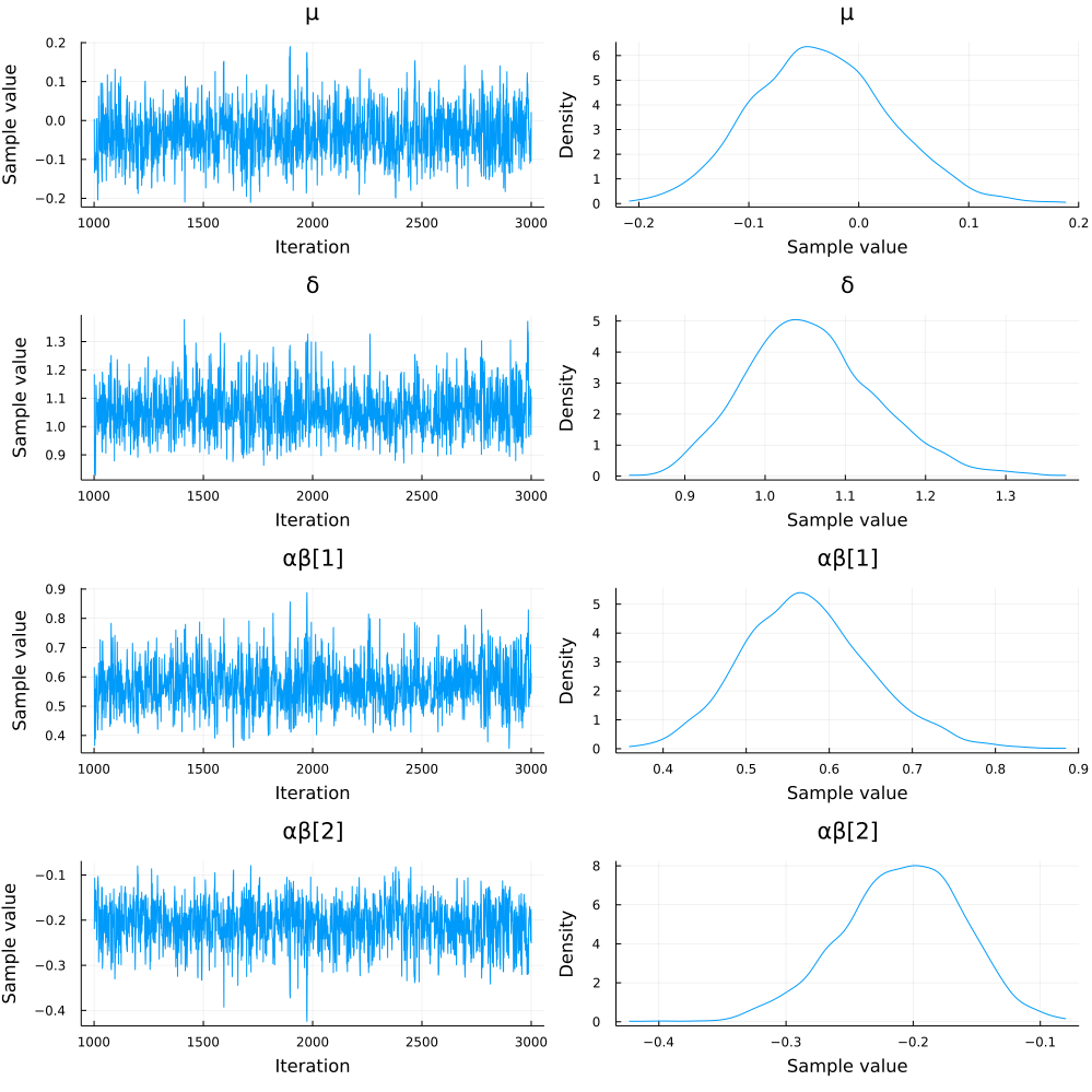
μ = 0
α = 0.5
β = -0.2
δ = 1

Random.seed!(1234)
data = rand(NormalInverseGaussian(μ, α, β, δ), 1_000)
model1 = nig1(data)
chain1 = Turing.sample(model1, NUTS(), 2_000)
plot(chain1)

I would also like to simulate from the posterior predictive distribtuion, but I am having trouble working with the predict function from Turing.

But what about using the definition of the NIG distribution? That should also alleviate the problem with the pdf. That is certainly possible:

@model function nig2(x)
    μ ~ Normal()
    δ ~ Exponential(1)
    αβ ~ CustomDist()
    α, β = αβ
    γ = sqrt(α^2 - β^2)

    z ~ filldist(InverseGaussian(δ/γ, δ^2), length(x))
    x ~ MvNormal(μ .+ β .* z, Diagonal(z))
end

chain2 = sample(nig2(data), NUTS(), 2_000)
parameter_names = names(chain2)
plot(chain2[parameter_names[1:4]])

This chunk was not run when generating this page. Whereas inference with nig1 takes about 1 minute (on my computer) inference with nig2 takes about 30 minutes.

In nig2 we also sample all the latent z variables; that may or may not be of interest. It it also the reason why we only plot a subset of the chain.