Bayesian inference for NIG with Stan

My last post was about Bayesian inference in the Normal-Inverse-Gaussian (NIG) distribution using Turing. But Turing is not the only PPL. Here I look into performing the same task with Stan.

One difficulty with Stan is that neither the NIG nor the inverse Gaussian distribution is available in Stan’s domain specific language, so I have to define the required functions myself. Stan needs the log pdf for inference and a random number generator for predictive distributions.

Consider the following Stan program saved as nig.stan.

functions {
    real ig_lpdf(real z, real delta, real gamma)
    {
        return log(delta) + gamma * delta - 0.5 * (3*log(z) + square(gamma)*z + square(delta)*inv(z));
    }

    // Random number generator for different parametrization:
    // https://github.com/JuliaStats/Distributions.jl/blob/master/src/univariate/continuous/inversegaussian.jl
    real ig_rng(real delta, real gamma)
    {
        real mu = delta * inv(gamma);
        real lambda = square(delta);

        real z = normal_rng(0, 1);
        real w = mu * square(z);
        real x1 = mu + mu * inv(2 * lambda) * (w - sqrt(w * (4 * lambda + w)));
        real p1 = mu * inv(mu + x1);
        real u = uniform_rng(0, 1);

        real y = u >= p1 ? square(mu) * inv(x1) : x1;
        return y;
    }
}


data {
    int<lower=1> N;
    vector[N] x;
}


parameters {
    real<lower=0> alpha;
    real<lower=-alpha, upper=alpha> beta;
    real mu;
    real<lower=0> delta;

    vector<lower=0>[N] z;
}


transformed parameters {
    real<lower=0> gamma = sqrt(alpha^2 - beta^2);
}


model {
    // Prior
    alpha ~ exponential(1);
    mu ~ normal(0, 1);
    delta ~ exponential(1);

    // Likelihood
    for (n in 1:N)
    {
        target += ig_lpdf(z[n] | delta, gamma);
        target += normal_lpdf(x[n] | mu + beta * z[n], sqrt(z[n]));
    }
}


generated quantities {
    real y;
    {
        real z_gen = ig_rng(delta, gamma);
        y = normal_rng(mu + beta * z_gen, sqrt(z_gen));
    }
}

In generated quantities we simulated observations from the posterior predictive distribution.

Compared to the Turing program it is much easier to enforce the bound \(|\beta| < \alpha\). Here I first define a model and later user rstan::sampling. It is also possible to call rstan::stan with the file instead.

nig_model <- rstan::stan_model(file = "nig.stan")

Now we simulate data from a NIG distribution using the {GeneralizedHyperbolic} package and simulate from the above model.

set.seed(1)
params <- c(mu = 0, delta = 1, alpha = 0.5, beta = -0.2)
n <- 2000
nig_data <- list(N = n, x = GeneralizedHyperbolic::rnig(n, param = params))

nig_fit <- rstan::sampling(nig_model, data = nig_data, chains = 1, iter = 2000, warmup = 1000)

## 
## SAMPLING FOR MODEL '2b56cb8cf0630e700f7c9a48c184a984' NOW (CHAIN 1).
## Chain 1: 
## Chain 1: Gradient evaluation took 0.002458 seconds
## Chain 1: 1000 transitions using 10 leapfrog steps per transition would take 24.58 seconds.
## Chain 1: Adjust your expectations accordingly!
## Chain 1: 
## Chain 1: 
## Chain 1: Iteration:    1 / 2000 [  0%]  (Warmup)
## Chain 1: Iteration:  200 / 2000 [ 10%]  (Warmup)
## Chain 1: Iteration:  400 / 2000 [ 20%]  (Warmup)
## Chain 1: Iteration:  600 / 2000 [ 30%]  (Warmup)
## Chain 1: Iteration:  800 / 2000 [ 40%]  (Warmup)
## Chain 1: Iteration: 1000 / 2000 [ 50%]  (Warmup)
## Chain 1: Iteration: 1001 / 2000 [ 50%]  (Sampling)
## Chain 1: Iteration: 1200 / 2000 [ 60%]  (Sampling)
## Chain 1: Iteration: 1400 / 2000 [ 70%]  (Sampling)
## Chain 1: Iteration: 1600 / 2000 [ 80%]  (Sampling)
## Chain 1: Iteration: 1800 / 2000 [ 90%]  (Sampling)
## Chain 1: Iteration: 2000 / 2000 [100%]  (Sampling)
## Chain 1: 
## Chain 1:  Elapsed Time: 33.3845 seconds (Warm-up)
## Chain 1:                19.932 seconds (Sampling)
## Chain 1:                53.3165 seconds (Total)
## Chain 1:

Time-wise this is comparable with the fast version in Turing, but much faster than the slow version that use the same sampling approach.

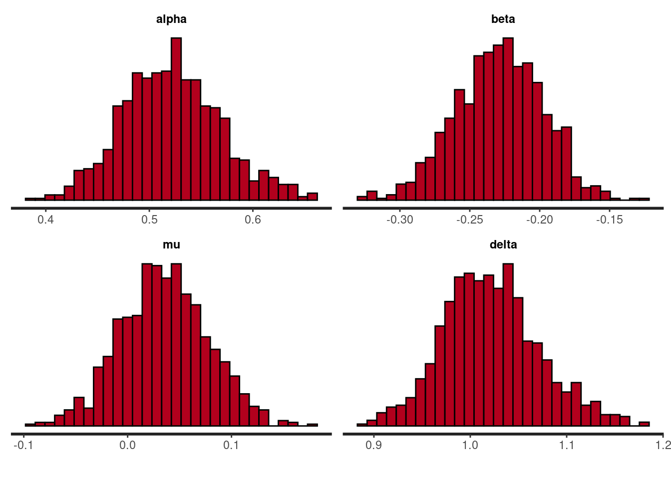
We can inspect the distribution of the parameters with functions from the {rstan} package (whose origin is the {bayesplot} package).

rstan::stan_hist(nig_fit, pars = c("alpha", "beta", "mu", "delta"))

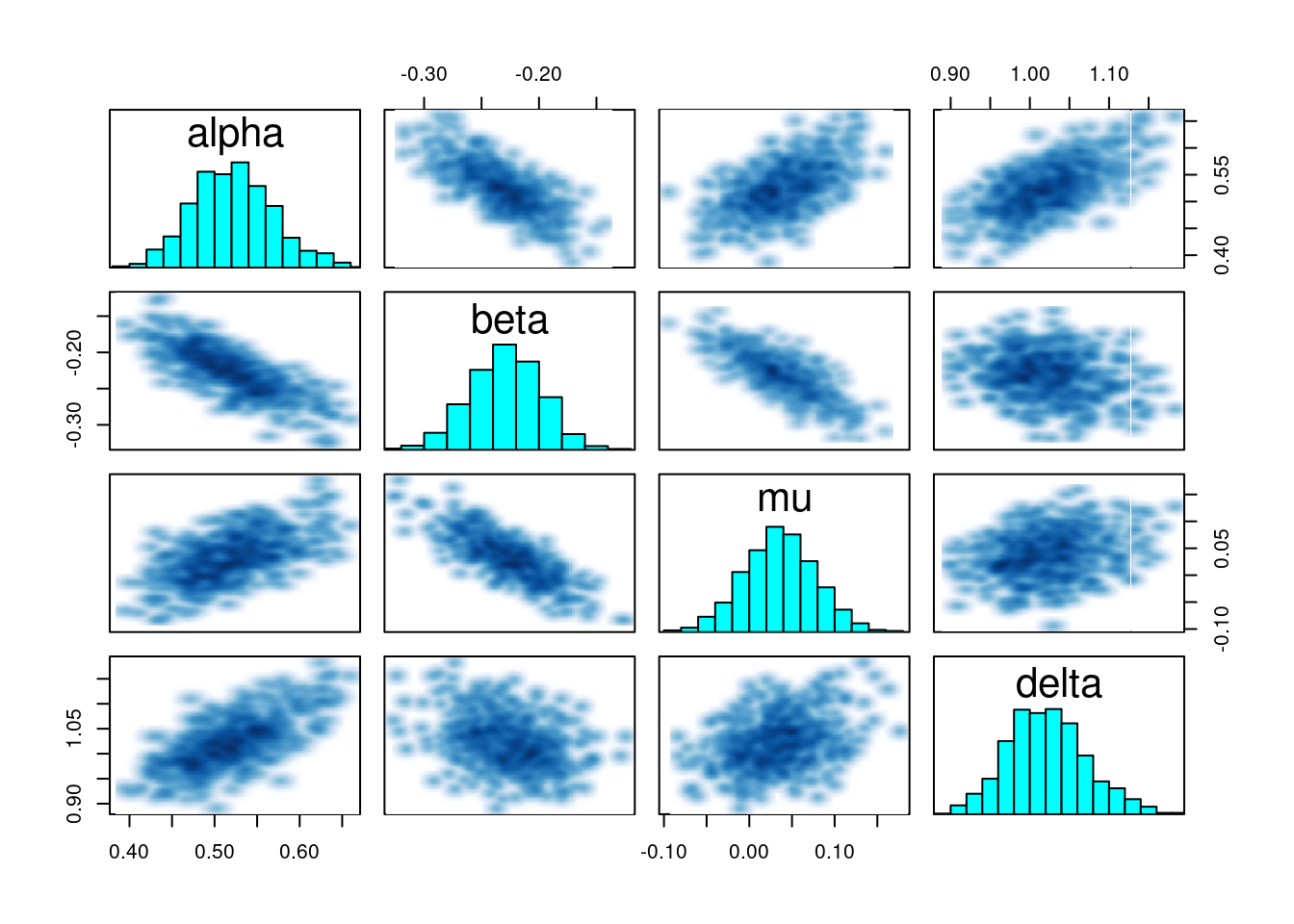
We can also visualize the pairwise joint distributions:

pairs(nig_fit, pars = c("alpha", "beta", "mu", "delta"))

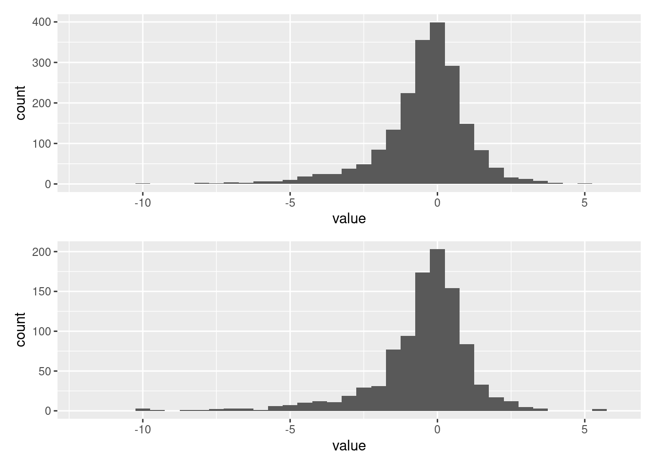
Finally a comparison of the data and simulations from the posterior predictive distribution

library(ggplot2)
library(patchwork)

simulated_data <- tibble::as_tibble(rstan::extract(nig_fit, pars = "y")$y)
simulated_plot <- ggplot(simulated_data, aes(value)) + 
    geom_histogram(binwidth = 0.5) + 
    xlim(-12, 6)

data_plot <- ggplot(tibble::as_tibble(nig_data$x), aes(value)) + 
    geom_histogram(binwidth = 0.5) + 
    xlim(-12, 6)

data_plot / simulated_plot