library(magrittr)
library(ggplot2)

Introduction

Let me first create some data to support my explanation. The data is meant to illustrate the prices of three financial futures, to be delivered in February, March and April, respectively.

prices <- tibble::tibble(
    Date = seq(from = as.Date("2020-01-01"), to = as.Date("2020-04-01"), by = 1),
    February = rnorm(length(Date), mean = 2),
    March = rnorm(length(Date), mean = 10),
    April = rnorm(length(Date), mean = 6)
)

The data is turned into “long” format to work better with ggplot:

prices_ts <- prices %>% 
    tidyr::pivot_longer(
        cols = c("February", "March", "April"), 
        names_to = "Contract", 
        values_to = "Price"
    ) %>% 
    dplyr::mutate(
        Price = dplyr::case_when(
            lubridate::month(Date, label = TRUE, abbr = FALSE) >= Contract ~ NA_real_,
            TRUE ~ Price
        )
    ) %>% 
    tidyr::drop_na() %>% 
    tsibble::tsibble(key = Contract, index = Date)

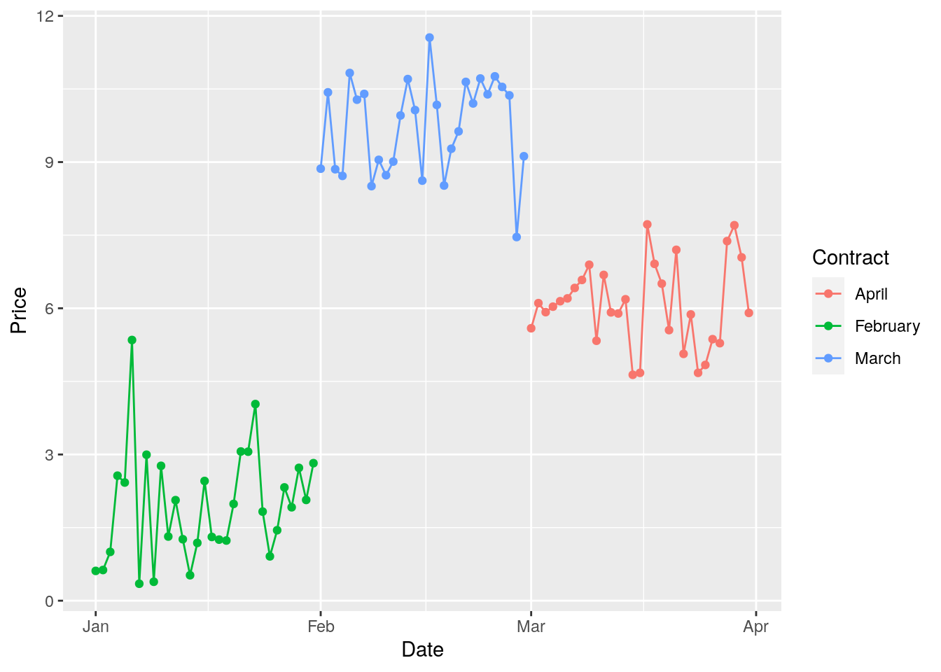
Plotting the tsibble we see that the futures are traded up to their delivery.

prices_ts %>% 
    ggplot(aes(Date, Price, group = Contract, color = Contract)) +
    geom_point() +
    geom_line()

A “rolled time series” is made by combining these three time series into a single time series.

The rolled time series of the “first front month” is made by taking the February prices in January, the March prices in February and the April prices in March.

Similarly, the time series of the “second front month” is made by taking the February prices in December, the March prices in January and the April prices in February.

The value of the “Nth front month” time series at time T is from the time series whose delivery date is between N - 1 and N months away.

This tRick is about how we can compute such rolled time series.

POSIXct vs POSIXlt

Let us first recall the difference betwwen the two datetime representations in R.

t <- lubridate::ymd_hms("2020-02-29 12:34:56")

The POSIXct representation of t is the number of seconds since the beginning of time:

unclass(t)

## [1] 1582979696
## attr(,"tzone")
## [1] "UTC"

In the POSIXlt representation of t every part is saved separately:

as.POSIXlt(t) %>% unlist() %>% unclass()

##   sec   min  hour  mday   mon  year  wday  yday isdst 
##    56    34    12    29     1   120     6    59     0

This is the reason why datetimes in tibbles/dataframes must be in POSIXct and not in POSIXlt.

Computing fronts

The POSIXlt comes to handy here, because it easily allows us to get the integer number of months between two datetimes without worrying about “modulo 12”.

First we get the number of months since a fixed origin:

number_of_months <- function(timestamp) { 
    lt_rep = as.POSIXlt(timestamp, origin = "1900-01-01")
    lt_rep$year*12 + lt_rep$mon
}

Then the number of months between two timestamps:

month_diff = function(t1, t2) { number_of_months(t1) - number_of_months(t2) }

Now we can compute which front month each observation belongs to (this computation of delivery date is of course only useful in this example):

prices_ts <- prices_ts %>% 
    dplyr::mutate(
        DeliveryDate = as.Date(paste(2020, match(Contract, month.name), 1, sep = "-")),
        Front = month_diff(DeliveryDate, Date)
    )
tibble::glimpse(prices_ts)

## Rows: 182
## Columns: 5
## Key: Contract [3]
## $ Date         <date> 2020-01-01, 2020-01-02, 2020-01-03, 2020-01-04, 2020-01…
## $ Contract     <chr> "April", "April", "April", "April", "April", "April", "A…
## $ Price        <dbl> 6.218993, 5.891068, 4.406832, 5.068562, 4.862892, 6.5360…
## $ DeliveryDate <date> 2020-04-01, 2020-04-01, 2020-04-01, 2020-04-01, 2020-04…
## $ Front        <dbl> 3, 3, 3, 3, 3, 3, 3, 3, 3, 3, 3, 3, 3, 3, 3, 3, 3, 3, 3,…

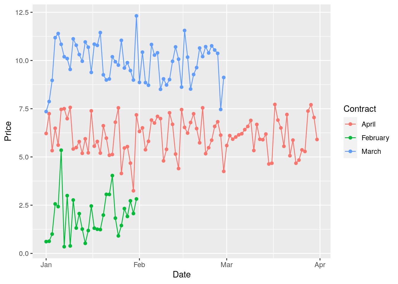
A plot with the rolled series with the first front month:

prices_ts %>% 
    dplyr::filter(Front == 1) %>% 
    ggplot(aes(Date, Price, group = Contract, color = Contract)) +
    geom_point() +
    geom_line()